Blog

Introduction

In the last post, Deep Anomaly Detection in Time Series (1) : Time Series Data, I introduced time series data and types of anomalies. In this post, I will introduce why anomaly detection is difficult and how to detect different types of anomalies.

In recent years, artificial intelligence has been making great strides. As a result, research in many fields, including image recognition, autonomous driving, speech-to-text, and text-to-speech, has seen dramatic results. A prime example is Image Classification, a field of artificial intelligence that attempts to determine what kind of image an image is when given an image as input. The ImageNet Large Scale Visual Recognition Challenge (ILSVRC)[1], which trains a million images to classify 150,000 new images into 1,000 categories, had an accuracy rate of about 50% in 2011, but now, 10 years later, it has an accuracy rate of over 90%.

Artificial intelligence is being industrialised in many fields with these remarkable achievements. However, the field of anomaly detection has yet to be industrialised due to its inherent complexity and challenges. So why is anomaly detection so difficult? Lukas et al[2] cite three reasons why anomaly detection is difficult.

If you look up the definition of the word “Anomaly”, you’ll find that it means “a state of being different from the usual”. In other words, any kind of pattern other than the usual data pattern (normal data) can be called anomalous data. There will be only a few kinds of normal data, but the patterns of anomalous data will be very diverse. Moreover, if the data is a multivariate time-series (see previous post), the diversity of anomalous patterns will increase exponentially. And with so many anomalous patterns, it is possible to encounter anomalous patterns that have never been seen before. This diversity will naturally make the problem difficult.

In a typical case, the number of data containing anomalous patterns will be very small compared to the normal data. When the proportions of data differ significantly, this is known as “data imbalance”, which makes it difficult to train anomaly detection models and, by extension, to actually detect them.

One of the most important things in training machine learning and deep learning models is the amount of data, and the following figure shows that the amount of data is important for traditional machine learning methods, but it is even more important for deep learning methods. On the other hand, in the anomaly detection problem, no matter how many normal data there are, it is difficult to get good anomaly detection performance because the important anomaly data are too few.

Data imbalance also causes difficulties in actual field application. Due to the nature of the anomaly detection problem, ‘classifying abnormal data as normal (Type 2 Error, False Negative)’ is more fatal than ‘classifying normal data as abnormal (Type 1 Error, False Positive)’. It is a highly difficult problem to find all the abnormal data in the data without missing it. However, if half of the normal data is classified as an anomaly, the meaning of anomaly detection is lost.

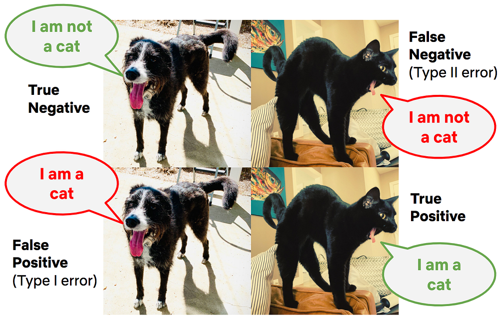
Examples of Type 1 and Type 2 errors (source: Netflix blog)

The types of anomaly data were covered in detail in the last post (Deep Anomaly Detection in Time Series (1): Time Series Data). Anomaly data can itself be divided into three types, called Point Anomaly, Contextual Anomaly, and Group Anomaly.

Each of these anomalous data has very different characteristics, so it can be said that it is difficult to detect all kinds of anomalous data. For more information on the types of abnormal data, please refer to the previous post.

There are many methods that have been researched in the field of anomaly detection in time series data for the problems mentioned above. It is not possible to introduce or categorise all of them in this article, but I would like to briefly introduce some of the methods that have been used in the past, their limitations, and alternative methods.

How has anomaly detection in time series data been done in the past? There are many, but here’s a quick overview of the top three: 3-sigma, boxplot, and ARIMA.

For 3-sigma, 99.7% of the data falls within 3 standard deviations (3σ) of a normal distribution, treating the rest as outliers, while boxplot uses quartiles and interquartile ranges to define outliers. Finally, ARIMA (Auto-regressive Integrated Moving Average) is often used to forecast time series.It is used for anomaly detection by predicting future time series and then determining anomalous data through the error of the observed data or the probability of the observed value occurring.

Univariate time series ARIMA (Source : https://github.com/Jenniferz28/Time-Series-ARIMA-XGBOOST-RNN)

However, all of these methods are for univariate time-series and have the disadvantage that Boxplot and 3-sigma can only detect Point Anomalies.

Among the three methods mentioned above, if ARIMA predicts time series data well, it can theoretically detect all three types of anomalies. However, we were limited to univariate time-series, so shouldn’t multivariate time-series also be able to detect anomalies through predic.

However, one of the most prestigious competitions in time series forecasting, the Makridakis competitions (M Competition) [5, 6], states that “the main purpose of forecasting is not to reduce uncertainty, but to show all possibilities as precisely as possible” and that “all forecasts are uncertain, and this uncertainty cannot be ignored”. This is why the 2020 competition was organised not only for Accuracy [5] but also for Uncertainty [6].

Therefore, for multivariate time series where the uncertainty is inevitably larger than univariate, prediction-based anomaly detection may not be of much help. However, if you have data with relatively small uncertainties and a model that can represent the uncertainties in a sophisticated way, prediction-based anomaly detection can be a valid option.

So, aside from predictive-based anomaly detection, what is the first method that comes to mind when you think of using artificial intelligence to detect anomalies in time-series data?

I think it’s probably a way to train an artificial intelligence model that classifies time series data into abnormal and normal. Deep learning models are also showing good results in the field of image classification. Learning by labeling anomalies/normals in advance for each data type is called ‘supervised learning’ (a time series prediction model is also a type of supervised learning).

If you create a supervised learning-based anomaly detection model, learning is like this: ‘data from 09:00 to 09:10 is normal, data from 09:10 to 09:20 is normal, data from 09:20 to 09:30 is abnormal’ I wonder if it will. If this learning is ideal, the model will be able to detect all three types of anomaly data (Point Anomaly, Contextual Anomaly, and Group Anomaly) with high accuracy. In fact, supervised learning is known to be the best performing method among artificial intelligence learning methods.

However, there is a big problem with this intuitive method. No matter how much data there is, only a fraction of it is anomalous, and it is difficult for humans to find and label such anomalies. In this situation, it is difficult to prepare the data, and even if it is prepared, the model is unlikely to learn well due to data imbalance.

But is there a way to do it without labelling? The method of learning from data without labelling is called ‘Unsupervised Learning’.

The most common of these is the Autoencoder-based model. An autoencoder consists of an encoder that compresses the input data into smaller dimensional data, and a decoder that restores the compressed data back to something close to the input data. This is illustrated below.

The concept of an autoencoder (Source: Wikipedia)

The most common of these is the Autoencoder-based model. An autoencoder consists of an encoder that compresses the input data into smaller dimensional data, and a decoder that restores the compressed data back to something close to the input data. This is illustrated below.

An example of representing high-dimensional data (left) as a low-dimensional manifold (right).

The anomalous data (marked with an X) is mapped by the Autoencoder and transformed into a manifold of normal data.

This manifold means “key features across the training data,” and it is difficult to include the features of anomalous data, which is a very small amount of data. So, if you put normal data into the Auto Encoder at the end of training, you will get a normal reconstructed output, but if you put anomalous data, the features of the anomalous data will not be extracted well, and you will get normal data that is closest to the input data. Then, the difference between the input data and the output data (Reconstruction Error) will be larger than the normal data, and this difference can be used to detect anomalous data.

If you create a model based on these autoencoders, the model can consider any data that does not have a normal pattern as anomalous data, regardless of the type or pattern of the anomaly. However, the manifold depends on many factors, including the structure of the model, which leads to ups and downs in performance. This means that performance can vary greatly depending on your model settings (hyperparameters), and it can be difficult to find the best performing model.

Also, if the anomaly data is close to the normal data, or can be represented by the same manifold, Autoencoder may be able to successfully recover even the anomalous data. If this happens, the anomaly detection model will not be able to detect it well.

So far, we’ve covered cases where normal/abnormal labelling is required for all data, and cases where labelling is not required. But what if you already know a large amount of normal data and a small amount of abnormal data? A method that learns by labelling only a subset of the total data is called ‘semi-supervised learning’. It’s a relatively new methodology compared to the other two (supervised and unsupervised).

One of the semi-supervised learning-based anomaly detection models is DeepSVDD[6]. It is a model that applies deep learning to SVDD (Support Vector Data Description). In brief, it converts data into a feature space, a space of only data features, but learns only normal data to find the optimal hypersphere surrounding normal features. Data inside this hypersphere is normal, and data outside is anomalous.

Concept of DeepSVDD: Data (left) is mapped to feature space (right) via a model (centre), where normal data is located inside the hypersphere and anomalous data is located outside the hypersphere.

This has been a brief introduction to anomaly detection in time series data. There is a lot of research going on in anomaly detection from different perspectives. Some of these areas include

• Out-of-Distribution (OD): a discipline that classifies different kinds of steady states, but still allows you to identify data as Unknown when you encounter it for the first time.
• Contrast Learning: An unsupervised learning method that learns the similarity of data without labels such as normal/abnormal to achieve accuracy comparable to supervised learning models.
• Generative Model: Apply a generative model such as VAE (Variational Autoencoder) or GAN (Generative Adversarial Network) to improve accuracy by learning the distribution of training data.
• Transformer: How to apply Transformer-based models, which have performed well in Natural Language Processing (NLP), to anomaly detection.

However, a significant number of these studies are aimed at anomaly detection in image data rather than time series data, so how can these models be applied to time series data?

Representative methods include STFT (Short-term Fourier Transform), CWT (Continuous Wavelet Transform), and nowadays, CQT (Constant Q Transform). In practice, when analysing time series data using an AI model, the data is pre-processed by various methods such as STFT, CWT, and others before being input to the AI model. This pre-processing of the data is called ‘preprocessing’. We’ll talk about preprocessing for time series data another time.

STFT (Source : Digital Signal Processing System Design)

So far, we’ve covered cases where normal/abnormal labelling is required for all data, and cases where labelling is not required. But what if you already know a large amount of normal data and a small amount of abnormal data? A method that learns by labelling only a subset of the total data is called ‘semi-supervised learning’. It’s a relatively new methodology compared to the other two (supervised and unsupervised).

Reference

• Ruff, Lukas, et al. “A unifying review of deep and shallow anomaly detection.” Proceedings of the IEEE (2021).
• Russakovsky, Olga, et al. “Imagenet large scale visual recognition challenge.” International journal of computer vision 115.3 (2015): 211-252.
• Makridakis, S., E. Spiliotis, and V. Assimakopoulos. “The M5 accuracy competition: Results, findings and conclusions.” Int J Forecast (2020).
• Makridakis, S., et al. “The M5 Uncertainty competition: Results, findings and conclusions.” International Journal of Forecasting (2020): 1-24.
• https://en.wikipedia.org/wiki/Autoencoder