Blog

Introduction

Recently, 4th Industrial Revolution technologies are being actively researched and applied in the fields of manufacturing management systems, smart factories, and predictive maintenance. Among them, “Anomaly Detection” is a key field for implementing AI and IoT technologies, and is based on the principle of data analysis and application.

As a DBMS specializing in time series databases, Machbase has the core and original technology for anomaly detection due to its long history of boasting the world’s №1 speed and performance in this field. In this post, I will give you an overview of Deep Anomaly Detection, the characteristics of time series data, and types of anomalies.

Let’s start by looking at Time Series data itself.

Time Series Data

we need to look at the data itself. Data called a time series, or time series, is a sequence of data placed at regular time intervals. What are the characteristics of this time series data? Let’s look at it from two perspectives.

First, let’s look at how time series data is organized. Time series data can be decomposed into Seasonality, Trend, and Remainder. Seasonality is a recurring pattern with short intervals throughout the time series data, Trend is the overall increase or decrease in the time series, and Remainder is the irregularities that cannot be explained by these two factors.

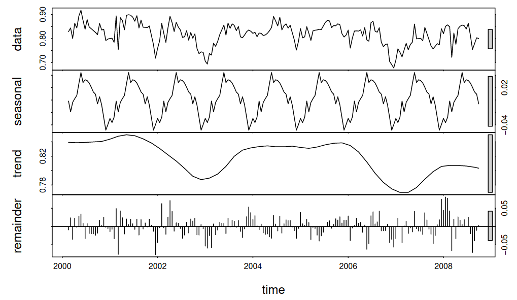
The organization of time series data: data consists of seasonality, trend, and residuals (1)

For example, temperature or gasoline engines (in some cases, seasonal changes may be included in the temperature data)

• Seasonality : temperature change according to day and night
• Trend : Changes in temperature due to weather and seasonal changes
• Remainder : Noise that cannot be expressed as Seasonality or Trend

• Seasonality : Periodic vibration changes due to intake, compression, explosion, and exhaust
• Trend : Changes in sensor values due to changes in vehicle speed, aging of vehicles, etc.
• Remainder : Noise that cannot be expressed as Seasonality or Trend

This process of identifying the type of time series data and categorizing it into Trend, Seasonality, and Remainder is called Time Series Decomposition. Time series decomposition can be done in two ways depending on the shape of the data: “Additive Model” and “Multiplicative Model”.

The Additive Model time series is the sum of Seasonality, Trend, and Remainder, and the Multiplicative Model time series is the product of the three.

In the time series of the Additive Model, the frequency and amplitude of the data are relatively constant even if the trend changes, but in the case of the Multiplicative Model, the frequency and amplitude change together as the trend of the data changes.

Additive Model & Multiplicative Model(2)

When predicting time series data, we can use decomposition to simplify the problem, but what about from a DAD perspective? We can think of a case where the remaining variance of the vibration sensor increases as the bearing attached to the vibration sensor ages, or the trend of the monthly average temperature increases abnormally due to global warming, or the seasonality that has always been the same is suddenly deviated from. In other words, it is important to understand the components of the time series even in anomaly detection problems.

This time, let’s categorize time series data according to the number of dependent variables. Let’s say you want to predict the weather. If you want to predict the temperature in Busan, you can use the temperature in the past and the temperature in the future. If you want to predict the wind speed, you can consider only the wind speed in the past and the wind speed in the future. When there is only one variable that depends on time, such as ‘time-temperature’ and ‘time-wind speed’, it is called a univariate time series.

However, weather cannot be predicted by temperature, wind speed, and precipitation in isolation: if it’s sunny, the temperature will rise, and if there’s a cold snap, the wind will pick up and the temperature will drop. It’s only when the weather, precipitation, humidity, and wind are combined that we can predict the weather. When each of these dependent variables is affected not only by time but also by other dependent variables to form a complex time series, it is called a Multivariate Time Series.

Example of a multivariate time series: Weather forecast for Busan from April 27 to April 29 (Korea Meteorological Administration)

Not surprisingly, multivariate time series are more difficult to analyze than univariate time series. Traditionally, ARIMA (Auto-Regressive Integrated Moving Average) models have been used for univariate time series, and VAR (Vector Auto-Regressive) models have been used for multivariate time series, but due to the complexity of multivariate time series, they are not very effective.

Nowadays, a lot of research has been done on deep learning, and it is possible to recognize patterns in complex problems, so there is a movement to solve the analysis of multivariate time series with deep learning.

So, what are the different types of anomalies in a time series? Different papers have different ways of categorizing time series anomalies, but in this article, I’ll introduce the three types that more papers have identified.

Point Anomaly

Data that completely deviates from the distribution of normal data is known as a point anomaly or global outlier. They are the most commonly thought of anomalies and also the most studied. For example, in the following image, you can see that the data corresponding to the red dots deviates significantly from the distribution of the rest of the data. These two red pieces of data can be referred to as Point Anomalies.

Example of a Point Anomaly (3)

Contextual Anomaly

Also known as a conditional anomaly.

It refers to data where there is nothing strange about the distribution of the data itself, but the flow or context of the data is not normal. It’s when you expect to see certain data at a certain point in time, but you get something else. For example, in the following graph.

Example of Contextual Anomaly (4)

Group Anomaly

Group Anomalies, or Collective Anomalies as they are also called, are data that looks normal at first glance when viewed in isolation. However, it’s the type of anomaly that looks abnormal when viewed as a group of data.

In the following image, we see a series of $75 payments over three days starting on July 14. If it was a single payment, you might treat it as normal, but if it’s the same payment over and over again over the course of several days, it’s obviously suspicious. Or, as another example, consider a vibration sensor whose graph is slightly but consistently trending upward. It might look normal when you look at a single or short-term data point, but if it’s consistently upward over the long term, shouldn’t you take a look at your device?

Group Anomaly : Detecting anomalies in credit card usage(4)

These are the three types of anomalies. There are still more difficulties in detecting group anomalies than point anomalies or contextual anomalies, but recently, there have been many studies to solve them with deep learning methods such as Variational AutoEncoders (VAE), Adversarial AutoEncoders (AAE), and Generative Adversarial Networks (GAN). If you want to apply anomaly detection for smart factories, you will need to consider all three types of anomalies and build a model.

Conclusion

Techniques for anomaly detection are constantly being developed, with faster and more accurate models becoming available. Deciding which models to use in real-world applications and in which data collection environments is crucial.

In addition, anomaly detection is being applied and utilized in various industries by utilizing artificial intelligence and the Internet of Things as a basic step for factory automation smart factories. In addition, it is very important to select a time series database that is specialized for this purpose by compensating for the limitations of data collection, processing, and analysis that occur in existing relational DBMSs. So far, we have covered various contents on anomaly detection, and we will see you next time with more good contents.

Thank you.

• Verbesselt, Jan, et al. “Detecting trend and seasonal changes in satellite image time series.” Remote sensing of Environment 114.1 (2010): 106-115.
• https://kourentzes.com/forecasting/2014/11/09/additive-and-multiplicative-seasonality/
• Talagala, Priyanga Dilini, et al. “Anomaly detection in streaming nonstationary temporal data.” Journal of Computational and Graphical Statistics 29.1 (2020): 13-27./li>
• Chalapathy, Raghavendra, and Sanjay Chawla. “Deep learning for anomaly detection: A survey.” arXiv preprint arXiv:1901.03407 (2019).