FFT()

Fast Fourier Transform

📌

To follow the examples smoothly, run the following query to prepare the table and data in advance.

CREATE TAG TABLE IF NOT EXISTS EXAMPLE (
    NAME VARCHAR(20) PRIMARY KEY,
    TIME DATETIME BASETIME,
    VALUE DOUBLE SUMMARIZED
);

Generate sample data

Open a new tql editor on the web UI, then copy the code below and run it.

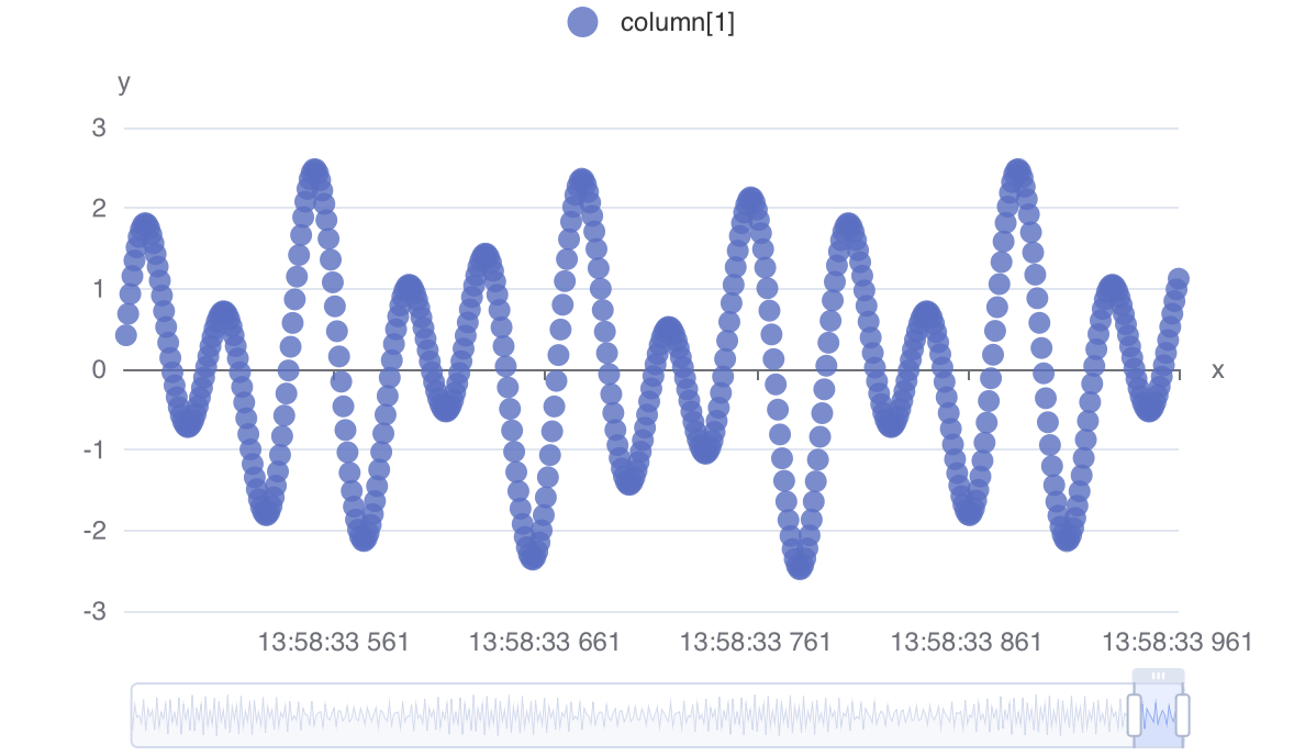
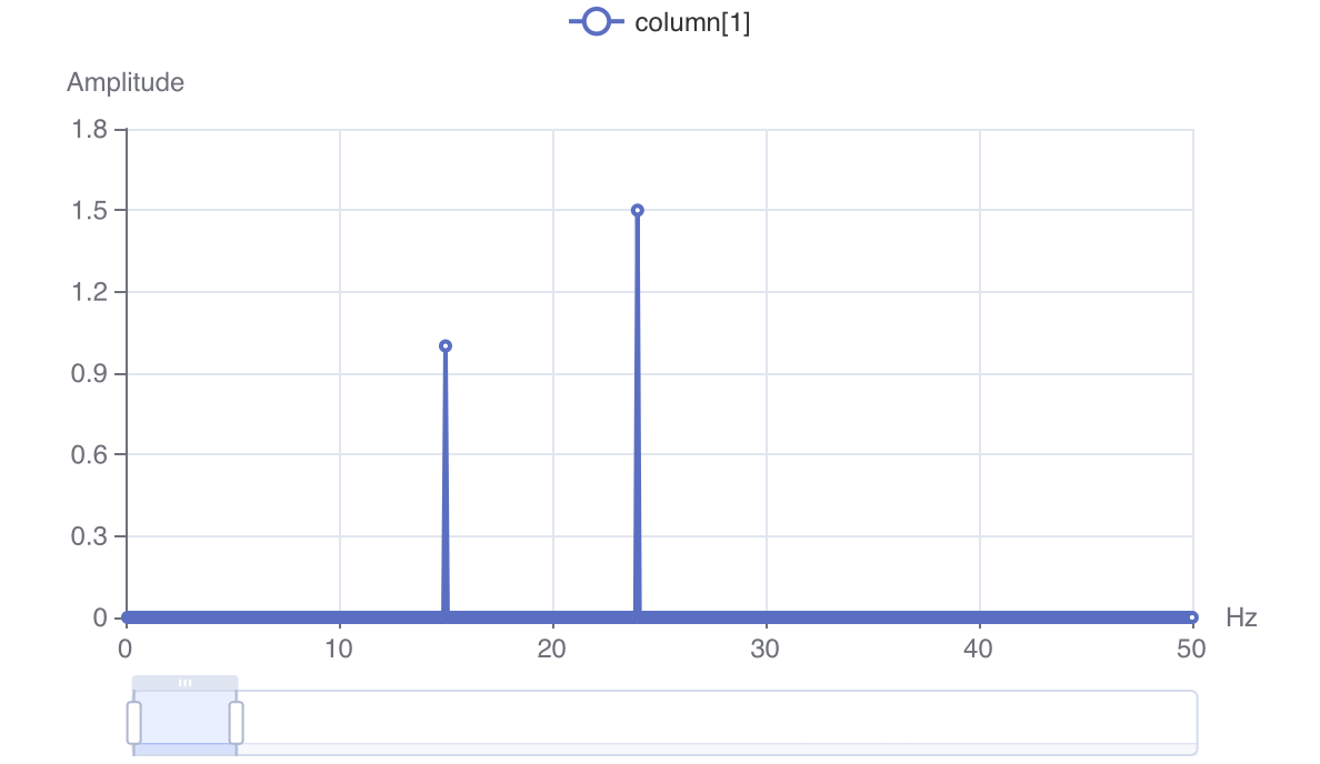
In this example, oscillator() generates a composite wave of 15Hz 1.0 + 24Hz 1.5. And CHART_SCATTER() has the dataZoom() option function that provides a slider under the x-axis.

 1
 2
 3
 4
 5
 6
 7
 8
 9
10
11
12
13
14
15
16
17
18
19
20
SCRIPT({
    const m = require('mathx');
    const data = m.oscillator({
        components: [
            { frequencyHz:15, amplitude:1.0 },
            { frequencyHz:24, amplitude:1.5 },
        ],
        timeRange: { from:"now", to:"now+10s"},
        sample:"1000Hz",
        noise: { amplitude: 0.3 },
    });
    const s = m.series(data, {xKey:"ts", yKey:"amp"})
    $.yield({
        xAxis:{ data: s.ts },
        yAxis: {},
        series: [ { type:"scatter", data: s.amp } ],
        dataZoom: { type: 'slider', start: 95, end: 100 },
    })
})
CHART( size("600px", "350px") )

Store data into database

Store the generated data into the database with the tag name ‘signal’.

 1
 2
 3
 4
 5
 6
 7
 8
 9
10
11
12
13
14
15
16
SCRIPT({
    const m = require('mathx');
    const data = m.oscillator({
        components: [
            { frequencyHz:15, amplitude:1.0 },
            { frequencyHz:24, amplitude:1.5 },
        ],
        timeRange: { from:"now", to:"now+10s"},
        sample:"1000Hz",
        noise: { amplitude: 0.3 },
    });
    for( d of data ) {
        $.yield(d[0], d[1]);
    }
})
SQL('insert into example values(?,?,?)','signal',value(0),value(1))

 1
 2
 3
 4
 5
 6
 7
 8
 9
10
FAKE(
  oscillator(
    freq(15, 1.0), freq(24, 1.5),
    range('now', '10s', '1ms')
  )
)
// |    0      1
// +--> time   magnitude
// |
SQL('insert into example values(?,?,?)','signal',value(0),value(1))

The “Result” pane shows 10000 rows inserted. for the FAKE example and 10001 rows inserted. for the SCRIPT example, because mathx.oscillator() includes both ends of the time range.

For reference, it took about 270ms on a test machine (Apple Mac mini M1), but using the APPEND() method in the example below took 65ms (x4 faster).

 1
 2
 3
 4
 5
 6
 7
 8
 9
10
11
12
13
14
15
16
SCRIPT({
    const m = require('mathx');
    const data = m.oscillator({
        components: [
            { frequencyHz:15, amplitude:1.0 },
            { frequencyHz:24, amplitude:1.5 },
        ],
        timeRange: { from:"now", to:"now+10s"},
        sample:"1000Hz",
        noise: { amplitude: 0.3 },
    });
    for( d of data ) {
        $.yield('signal', d[0], d[1]);
    }
})
APPEND( table('example') )

 1
 2
 3
 4
 5
 6
 7
 8
 9
10
11
12
13
14
FAKE(
  oscillator(
    freq(15, 1.0), freq(24, 1.5),
    range('now', '10s', '1ms')
  )
)
// |    0      1
// +--> time   magnitude
// |
PUSHVALUE(0,'signal')
// |    0         1      2
// +--> 'signal' time   magnitude
// |
APPEND( table('example') )

APPEND works only when the fields of input records exactly match the columns of the table in order and types.

Read data from database

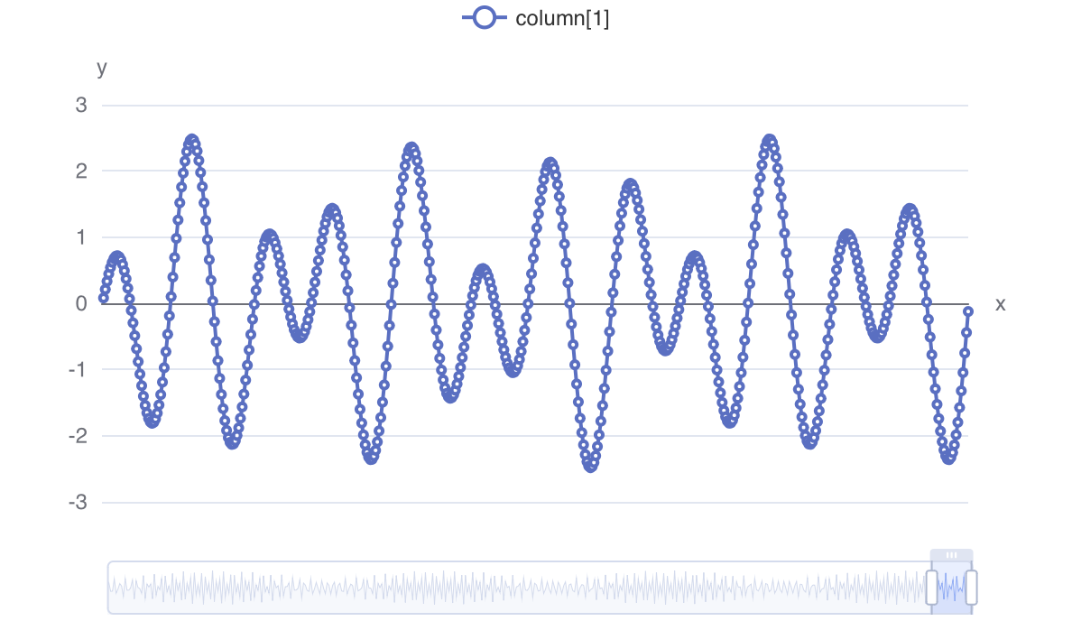
The code below reads the stored data from the ’example’ table.

SQL(`select time, value from example where name = 'signal' order by time`)
CHART(
    size("600px", "350px"), 
    chartOption({
        xAxis:{ data: column(0) },
        yAxis:{},
        series:[ {type:"line", data: column(1), showAllSymbol:true } ],
        dataZoom:{type:"slider", start:95, end: 100},
    })
)

Performing the Fast Fourier Transform

Add a few data transformation functions between the SQL_SELECT() source and the CHART_LINE() sink.

 1
 2
 3
 4
 5
 6
 7
 8
 9
10
SQL(`select time, value from example where name = 'signal' order by time`)
MAPKEY('sample')
GROUPBYKEY()
FFT()
CHART_LINE(
  size("600px", "350px"), 
  xAxis(0, 'Hz'),
  yAxis(1, 'Amplitude'),
  dataZoom('slider', 0, 10) 
)

 1
 2
 3
 4
 5
 6
 7
 8
 9
10
11
12
13
14
15
16
17
18
19
20
21
22
SQL(`select time, value from example where name = 'signal' order by time`)
SCRIPT({
    var times = [];
    var values = [];
},{
    ts = $.values[0];
    val = $.values[1];
    times.push(ts);
    values.push(val);
},{
    const mx = require("mathx");
    const result = mx.fft(times, values);
    const s = mx.series(result, {xKey:"freq", yKey:"amp"});
    $.yield({
        xAxis:{ name: "Hz", data: s.freq, axisLabel:{ }},
        yAxis:{ name: "Amplitude" },
        series:[ { type:"line", data: s.amp} ],
        dataZoom: { type:"slider", start: 0, end: 10 },
        tooltip:{ trigger: "axis" },
    });
})
CHART(size("600px", "350px"))

 1
 2
 3
 4
 5
 6
 7
 8
 9
10
11
12
13
14
15
16
17
18
19
20
21
22
SQL(`select time, value from example where name = 'signal' order by time`)
SCRIPT({
    var times = [];
    var values = [];
},{
    ts = $.values[0];
    val = $.values[1];
    times.push(ts);
    values.push(val);
},{
    const mx = require("mathx");
    result = mx.fft(times, values);
    for(i = 0; i < result.length; i++) {
        $.yield(...result[i]);
    }
})
CHART_LINE(
  size("600px", "350px"), 
  xAxis(0, 'Hz'),
  yAxis(1, 'Amplitude'),
  dataZoom('slider', 0, 10) 
)

How it works

SQL_SELECT()

SQL_SELECT(...) yields records from the query result in the form of {key: rownum, value: (time, value)}.

MAPKEY(‘sample’)

MAPKEY('sample') sets the constant string ‘sample’ as a new key for all records. As a result, all records have the same key 'sample' and (time, value) as value. {key: 'sample', value:(time, value)}

GROUPBYKEY()

GROUPBYKEY() merges all records that have the same key. In this example, all query results are combined into a record whose key is ‘sample’ and whose value is an array of tuples: {key: 'sample', value:[ (time1, value1), (time2, value2), ..., (timeN, valueN) ]}.

FFT()

FFT() applies the Fast Fourier Transform on the value of the record and transforms the array of (time, value) tuples into an array of (frequency, amplitude) tuples. {key: 'sample', value:[ (Hz1, Ampl1), (Hz2, Ampl2), ... ]}

Adding time axis

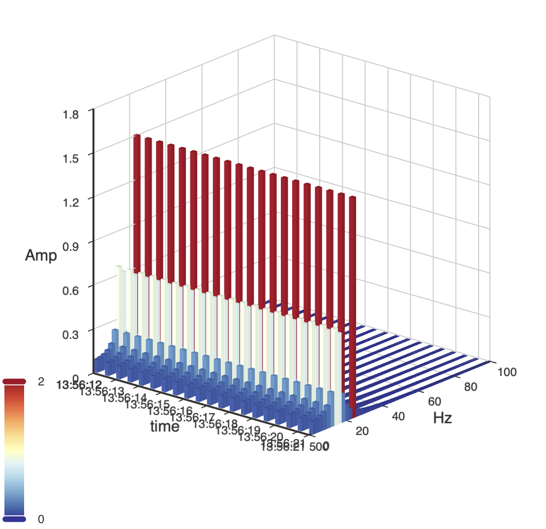
The following example adds a time axis to visualize the frequency transform results as a time series.

 1
 2
 3
 4
 5
 6
 7
 8
 9
10
11
12
13
SQL(`select time, value from example where name = 'signal' order by time`)

MAPKEY( roundTime(value(0), '500ms') )
GROUPBYKEY()
FFT(minHz(0), maxHz(100))
FLATTEN()
PUSHKEY('fft')
CHART_BAR3D(
      xAxis(0, 'time', 'time'),
      yAxis(1, 'Hz'),
      zAxis(2, 'Amp'),
      size('600px', '600px'), visualMap(0, 1.5), theme('westeros')
)

To query the 10 seconds up to the latest record of the tag with SQL_SELECT(), write the script as follows.

 1
 2
 3
 4
 5
 6
 7
 8
 9
10
11
12
13
SQL_SELECT( 'time', 'value', from('example', 'signal'), between('last-10s', 'last'))

MAPKEY( roundTime(value(0), '500ms') )
GROUPBYKEY()
FFT(minHz(0), maxHz(100))
FLATTEN()
PUSHKEY('fft')
CHART_BAR3D(
      xAxis(0, 'time', 'time'),
      yAxis(1, 'Hz'),
      zAxis(2, 'Amp'),
      size('600px', '600px'), visualMap(0, 1.5), theme('westeros')
)

How the time axis example works

SQL_SELECT()

SQL_SELECT(...) yields records from the query result in the form of {key: rownum, value: (time, value)}.

MAPKEY()

MAPKEY( roundTime(value(0), '500ms')) sets the new key to value(0) truncated to a 500-millisecond boundary. As a result, the records are transformed into {key: (time/500ms)*500ms, value:(time, value)}.

GROUPBYKEY()

GROUPBYKEY() groups the records in every 500ms. {key: time1In500ms, value:[(time1, value1), (time2, value2)...]}

FFT()

FFT() applies the Fast Fourier Transform to each record. The optional functions minHz(0) and maxHz(100) limit the scope of the output for better visualization. {key:time1In500ms, value:[(Hz1, Ampl1), ...]}, {key:'time2In500ms', value:[(Hz1, Ampl1), ...]}, …

FLATTEN()

FLATTEN() reduces the dimension of the value array by splitting it into multiple records. As a result, each frequency-amplitude pair is yielded as a separate record.

PUSHKEY()

PUSHKEY('fft') sets the constant string ‘fft’ as the new key for all records, and the previous key is “pushed” into the first place of the value array. {key:'fft', value:(time1In500ms, Hz1, Ampl1)}, {key:'fft', value:(time1In500ms, Hz2, Ampl2)}…

Last updated on Sep 21, 2026

GROUP()Noise Filters