GROUP()

Syntax

GROUP( [lazy(boolean)] [, by()] [, aggregator...] )

• lazy(boolean) set lazy mode (default: false)
• by(value [, timewindow()] [, name]) specify how to make group with given value. by() was mandatory in GROUP() but it has become an optional Since v8.0.14 to apply aggregator on the whole data in a time.
• aggregator list of aggregator, comma separated multiple functions are possible.

 1
 2
 3
 4
 5
 6
 7
 8
 9
10
11
12
13

FAKE(json({
    ["A", 1],
    ["A", 2],
    ["B", 3],
    ["B", 4]
}))
GROUP(
    by( value(0), "CATEGORY" ),
    avg( value(1), "AVG" ),
    sum( value(1), "SUM"),
    first( value(1) * 10, "x10")
)
CSV( header(true) )

Result

by()

by() takes value as the first argument and optionally timewindow() and name.

Syntax: by( value [, timewindow] [, label] )

• value grouping value, usually it might be time.
• timewindow(from, until, period) timewindow option.
• label string set new column label, (default “GROUP”)

lazy()

Syntax: lazy(boolean)

If it set false which is default, GROUP() works comparing the value of by() of the current record to the other value of previous record, if it founds the value has been changed, then produces new record. As result it can make a group only if the continuous records have a same value of by(). If lazy(true) is set, GROUP() waits the end of the input stream before yield any record to collecting all records, so that un-sorted by() value can be grouped, but it causes heavy memory consumption.

timewindow()

Syntax: timewindow( from, until, period ) Since v8.0.13

• from, until time are the time range. Note that from is inclusive and until is exclusive. Regardless of the existence of actual data, you can specify the desired time range.
• period duration represents the time interval between from and until.

See the timewindow example

aggregator

If no aggregator is specified GROUP make new array of the raw records for a each group by default. Takes multiple continuous records that have same value of by(), then produces a new record which have value array contains all individual values. For example, if an original records was {key:k, value:[v1, v2]}, {key:k, value:{v3, v4}}…{key:k, value:{vx, vy}}, GROUP( by(key()) ) produces the new record as {key:k, value:[[v1,v2],[v3,v4],...,[vx,vy]]}.

Aggregator

Syntax: function_name( value [, value...] [, where()] [, nullValue()] [, predict()] [, label])

• value one or more values depends on the function.
• where( predicate ) take boolean expression for the predication.
• nullValue(alternative) specify alternative value to use instead of NULL when the aggregator has no value to produce.
• predict(algorithm) specify an algorithm to predict value to use instead of NULL when the aggregator has no value to produce.
• label string set the label of the column (default is the name of aggregator function).

There are two types of aggregator functions, Type 1 functions only keep the final candidate value for the result. Type 2 functions hold the whole data of a group, it uses the data to produce the result of the aggregation then release memory for the next group. If GROUP() use lazy(true) and Type 2 functions together, it holds the entire input data of the related columns.

Options

where(), nullValue(), predict() and label arguments are the optional and it represents the option of the each function syntax description below.

where()

Syntax: where(predicate) Since v8.0.13

See the where example

nullValue()

Syntax: nullValue(alternative) Since v8.0.13

See the nullValue example

predict()

Syntax: predict(algorithm) Since v8.0.13

See the predict example

Functions

avg()

Type 1, Syntax: avg(x [, option...])

Average of the values in a group.

sum()

Type 1, Syntax: sum(x [, option...])

Total sum of the values in a group.

count()

Type 1, Syntax: count(x [, option...]) Since v8.0.13

Count of the values in a group.

first()

Type 1, Syntax: first(x [, option...])

The first value of the group.

last()

Type 1, Syntax: last(x [, option...])

The last value of the group.

min()

Type 1, Syntax: min(x [, option...])

The smallest value of the group.

max()

Type 1, Syntax: max(x [, option...])

The largest value of the group.

rss()

Type 1, Syntax: max(x [, option...])

Root sum square

rms()

Type 1, Syntax: rms(x [, option...])

Root mean square

list()

Type 2, Syntax: list(x [, option...]) Since v8.0.15

• x float value

list() aggregates the all x values and produce a single list which contians the individual values.

1
2
3
4
5
6

FAKE(json({["A",1], ["A",2], ["B",3], ["B",4], ["C",5]}))
GROUP(
    by(value(0)),
    list(value(1))
)
JSON()

{
    "data":{
        "columns":["GROUP","LIST"],
        "types":["string","float64"],
        "rows":[
            ["A",[1,2]],
            ["B",[3,4]],
            ["C",[5]]
        ]
    },
    "success":true,
    "reason":"success",
    "elapse":"220.375µs"
}

1
2
3
4
5
6
7

FAKE(json({["A",1], ["A",2], ["B",3], ["B",4], ["C",5]}))
GROUP(
    by(value(0),"name"),
    avg(value(1), "avg"),
    list(value(1), "values")
)
JSON(rowsArray(true))

{
    "data": {
        "columns": ["name", "values", "avg"],
        "types": [ "string", "list", "float64" ],
        "rows": [
            {  "name": "A", "avg": 1.5, "values": [ 1, 2 ] },
            {  "name": "B", "avg": 3.5, "values": [ 3, 4 ] },
            {  "name": "C", "avg": 5,  "values": [ 5 ] }
        ]
    },
    "success": true,
    "reason": "success",
    "elapse": "270.25µs"
}

1
2
3
4
5
6
7
8

FAKE(json({["A",1], ["A",2], ["B",3], ["B",4], ["C",5]}))
GROUP(
    by(value(0)),
    list(value(1))
)
POPVALUE(0)
FLATTEN()
JSON()

{
    "data": {
        "columns": ["LIST"],
        "types": ["list"],
        "rows": [
            [1,2],
            [3,4],
            [5]
        ]
    },
    "success": true,
    "reason": "success",
    "elapse": "252.625µs"
}

lrs()

Type 2, Syntax: lrs(x, y [, weight(w)] [, option...]) Since v8.0.13

• x float or time
• y float value
• weight(w) if omitted then all of the weights are 1.

Linear Regression Slope, assuming x-y is a point on a othogonal coordinate system. x can be number or time type.

mean()

Type 2, Syntax: mean(x [, weight(w)] [, option...])

• x float value
• weight(w) if omitted then all of the weights are 1.

mean() computes the weighted mean of the grouped values. If all of the weights are 1, use the lightweight avg() for the performance.

mean($x$, weight($w$)) = $ \frac{\sum {w_i x_i}} {\sum {w_i}} $

cdf()

Type 2, Syntax: cdf(x, q [, weight(w)] [, option...]) Since v8.0.14

• x float
• q float
• weight(w) if omitted then all of the weights are 1.

cdf() returns the empirical cumulative distribution function value of x, that is the fraction of the samples less than or equal to q. cdf() is theoretically the inverse of the quantile() function, though it may not be the actual inverse for all values q.

correlation()

Type 2, Syntax: correlation(x, y [, weight(w)] [, option...]) Since v8.0.14

• x, y float value
• weight(w) if omitted then all of the weights are 1.

correlation() returns the weighted correlation between the samples of x and y.

correlation($x$, $y$, weight($w$)) = $ \frac{\sum {w_i (x_i - \bar{x}) (y_i - \bar{y})}} {stdX * stdY} $, ($\bar{x}$ = mean x, $\bar{y}$ = mean y)

covariance()

Type 2, Syntax: covariance(x, y [, weight(w)] [, option...]) Since v8.0.14

• x, y float value
• weight(w) if omitted then all of the weights are 1.

covariance() returns the weighted covariance between the samples of x and y.

covariance($x$, $y$, weight($w$)) = $ \frac{\sum {w_i (x_i - \bar{x}) (y_i - \bar{y})}} { \sum {w_i} -1 } $, ($\bar{x}$ = mean x, $\bar{y}$ = mean y)

quantile()

Type 2, Syntax: quantile(x, p [, weight(w)] [, option...]) Since v8.0.13

• x float value
• p float fraction
• weight(w) if omitted then all of the weights are 1.

quantile() returns the sample of x such that x is greater than or equal to the fraction p of samples, p should be a number between 0 and 1.

It returns the lowest value q for which q is greater than or equal to the fraction p of samples

quantileInterpolated()

Type 2, Syntax: quantileInterpolated(x, p [, weight(w)] [, option...]) Since v8.0.13

• x float value
• p float fraction
• weight(w) if omitted then all of the weights are 1.

quantile() returns the sample of x such that x is greater than or equal to the fraction p of samples, p should be a number between 0 and 1.

The return value is the linearly interpolated.

median()

Type 2, Syntax: median(x [, weight(w)] [, option...])

• x float value
• weight(w) if omitted then all of the weights are 1.

Equivalent to quantile(x, 0.5 [, option...])

medianInterpolated()

Type 2, Syntax: medianInterpolated(x [, weight(w)] [, option...])

• x float value
• weight(w) if omitted then all of the weights are 1.

Equivalent to quantileInterpolated(x, 0.5 [, option...])

stddev()

Type 2, Syntax: stddev(x [, weight(w)] [, option...])

• weight(w) if omitted then all of the weights are 1.

stddev() returns the sample standard deviation.

stderr()

Type 2, Syntax: stderr(x [, weight(w)] [, option...])

• weight(w) if omitted then all of the weights are 1.

stderr() returns the standard error in the mean with stddev of the given values.

entropy()

Type 2, Syntax: entropy(x [, option...])

Shannon entropy of a distribution. The natural logarithm is used.

mode()

Type 2, Syntax: mode(x [, weight(w)] [, option...])

• weight(w) if omitted then all of the weights are 1.

mode() returns the most common value in the dataset specified by value and the given weights. Strict float64 equality is used when comparing values, so users should take caution. If several values are the mode, any of them may be returned.

moment()

Type 2, Syntax: moment(x, n [, weight(w)] [, option...]) Since v8.0.14

• x float64 value
• n float64 moment
• weight(w) if omitted then all of the weights are 1.

moment() computes the weighted n-th moment of the samples.

variance()

Type 2, Syntax: variance(x [, weight(w)] [, option...]) Since v8.0.14

• x float value
• weight(w) if omitted then all of the weights are 1.

variance() computes the unbiased weighted variance of the grouped values. When weights sum to 1 or less, a biased variance estimator should be used.

1
2
3
4
5
6

FAKE(json({[8,2], [2,2], [-9,6], [15,7], [4,1]}))
GROUP(
    variance(value(0), "VARIANCE"),
    variance(value(0), weight(value(1)), "WEIGHTED VARIANCE")
)
CSV(heading(true), precision(4))

Examples

timewindow()

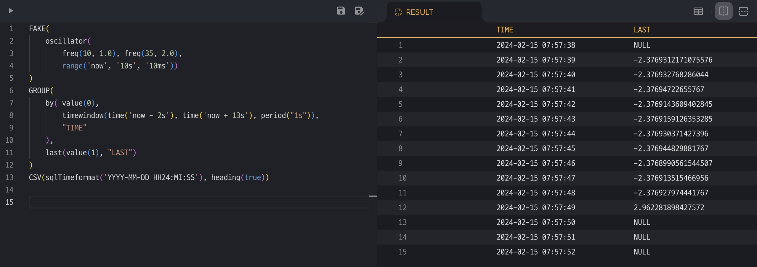
FAKE() generates time-value at every 1ms, so there are 1,000 records within 1 second. Executing the below TQL produces data at 1-second intervals (period("1s") in timewindow()), and if there is no actual data (record) in the desired time period, it is filled with the default value NULL.

 1
 2
 3
 4
 5
 6
 7
 8
 9
10
11
12
13
14
15

FAKE(
    oscillator(
        freq(10, 1.0), freq(35, 2.0), 
        range('now', '10s', '10ms')) 
)
GROUP(
    by( value(0),
        timewindow(time('now - 2s'), time('now + 13s'), period("1s")),
        "TIME"
    ),
    last( value(1),
          "LAST"
    )
)
CSV(sqlTimeformat('YYYY-MM-DD HH24:MI:SS'), heading(true))

nullValue()

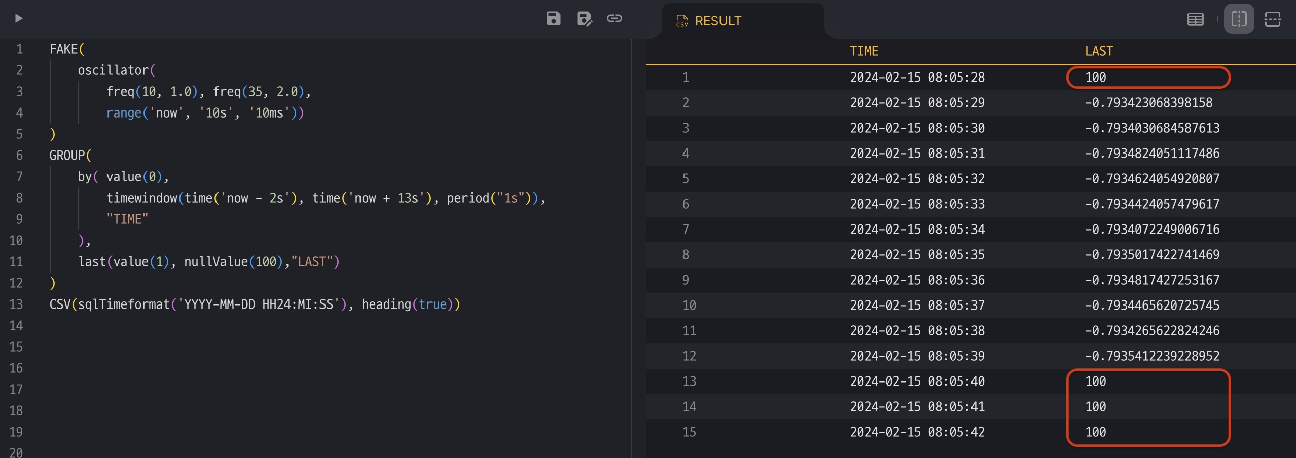
Let’s add nullValue(100) and execute again. The NULL values are replaced with the given value 100.

 1
 2
 3
 4
 5
 6
 7
 8
 9
10
11
12
13
14
15
16

FAKE(
    oscillator(
        freq(10, 1.0), freq(35, 2.0), 
        range('now', '10s', '10ms')) 
)
GROUP(
    by( value(0),
        timewindow(time('now - 2s'), time('now + 13s'), period("1s")),
        "TIME"
    ),
    last( value(1),
          nullValue(100),
          "LAST"
    )
)
CSV(sqlTimeformat('YYYY-MM-DD HH24:MI:SS'), heading(true))

predict()

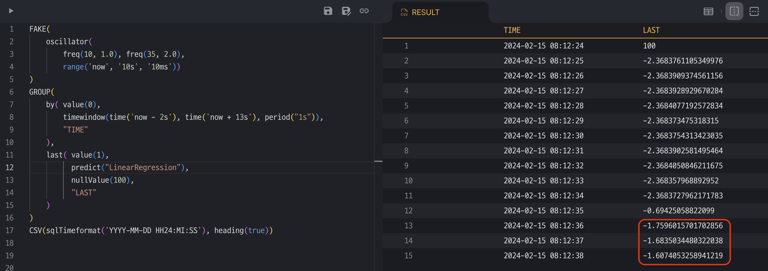
It is possible to obtain interpolated data by referring to adjacent values beyond filling empty values (NULL) with a constant specified by nullValue(). Using the example above, add predict("LinearRegression") to last() and execute it again. You can see that the value predicted by Linear Regression is filled in the records where NULL was returned because there was no value.

The predict() may fail to produce interpolation value when there are not enough values nearby to predict, then the nullValue() is applied instead. If nullValue() is not given, then NULL is returned.

 1
 2
 3
 4
 5
 6
 7
 8
 9
10
11
12
13
14
15
16
17

FAKE(
    oscillator(
        freq(10, 1.0), freq(35, 2.0), 
        range('now', '10s', '10ms')) 
)
GROUP(
    by( value(0),
        timewindow(time('now - 2s'), time('now + 13s'), period("1s")),
        "TIME"
    ),
    last( value(1),
          predict("LinearRegression"),
          nullValue(100),
          "LAST"
    )
)
CSV(sqlTimeformat('YYYY-MM-DD HH24:MI:SS'), heading(true))

where()

Let’s say there are two sensors that measure temperature and humidity, each one store the data per every 1 sec. In real world, there is always time difference among the sensor systems. So the stored data might be below samples.

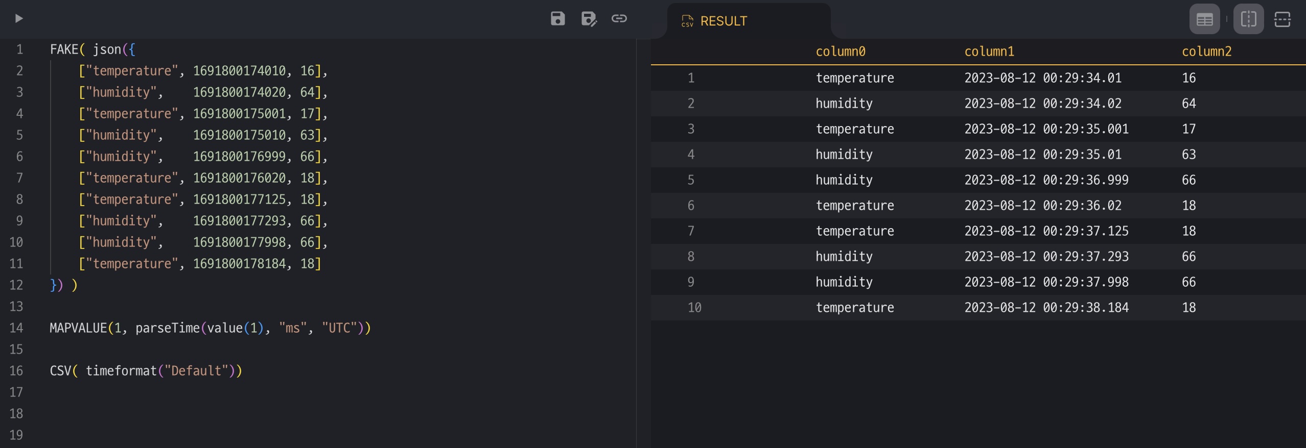
Record #5 humidity data store earlier than expect and it happens on record #9 again. Let’s normalize the data in second precision.

 1
 2
 3
 4
 5
 6
 7
 8
 9
10
11
12
13
14
15
16
17
18
19
20

FAKE( json({
    ["temperature", 1691800174010, 16],
    ["humidity",    1691800174020, 64],
    ["temperature", 1691800175001, 17],
    ["humidity",    1691800175010, 63],
    ["humidity",    1691800176999, 66],
    ["temperature", 1691800176020, 18],
    ["temperature", 1691800177125, 18],
    ["humidity",    1691800177293, 66],
    ["humidity",    1691800177998, 66],
    ["temperature", 1691800178184, 18]
}) )
MAPVALUE(1, parseTime(value(1), "ms"))

GROUP(
    by( roundTime(value(1), "1s")),
    avg( value(2) )
)

CSV( timeformat("Default"), header(true) )

roundTime(..., "1s") makes time value aligned in second, then make records grouped that has same time. avg(...) produces the average value of a group.

But it lost the first column information that indicates if the value is temperature or humidity, so the result values become meaningless. To solve this problem use where(). Aggregator functions accept values only when where() has the predicate true.

15
16
17
18
19
20
21
22
23

GROUP(
    by( roundTime(value(1), "1s"), "TIME"),
    avg( value(2),
         where( value(0) == 'temperature' ),
         "TEMP" ),
    avg( value(2),
         where( value(0) == 'humidity' ),
         "HUMI" )
)

It is also possible to interpolate the missing data of the last record with predict() and nullValue()

15
16
17
18
19
20
21
22
23
24

GROUP(
    by( roundTime(value(1), "1s"), "TIME"),
    avg( value(2),
         where( value(0) == 'temperature' ),
         "TEMP" ),
    avg( value(2),
         where( value(0) == 'humidity' ),
         predict("PiecewiseLinear"),
         "HUMI" )
)

Chart

 1
 2
 3
 4
 5
 6
 7
 8
 9
10
11
12
13
14
15
16
17
18
19
20
21
22
23

CSV(file("https://docs.machbase.com/assets/example/iris.csv"))
FILTER( strToUpper(value(4)) == "IRIS-SETOSA")
GROUP( by(value(4)), 
    min(value(0), "Min"),
    median(value(0), "Median"),
    avg(value(0), "Avg"),
    max(value(0), "Max"),
    stddev(value(0), "StdDev.")
)
CHART(
    chartOption({
        "xAxis": { "type": "category", "data": ["iris-setosa"]},
        "yAxis": {},
        "legend": {"show": "true"},
        "series": [
            {"type":"bar", "name": "Min", "data": column(1)},
            {"type":"bar", "name": "Median", "data": column(2)},
            {"type":"bar", "name": "Avg", "data": column(3)},
            {"type":"bar", "name": "Max", "data": column(4)},
            {"type":"bar", "name": "StdDev.", "data": column(5)}
        ]
    })
)

Result